Getting Started with workboots
Source:vignettes/Getting-Started-with-workboots.Rmd
Getting-Started-with-workboots.RmdSometimes, we want a model that generates a range of possible outcomes around each prediction. Other times, we just care about point predictions and may be able to use a powerful model. workboots allows us to get the best of both worlds — getting a range of predictions while still using powerful model!
In this vignette, we’ll walk through the entire process of building a boosted tree model to predict the range of possible car prices from the modeldata::car_prices dataset. Prior to estimating ranges with workboots, we’ll need to build and tune a workflow. This vignette will walk through several steps:
- Building a baseline model with default parameters.
- Tuning and finalizing model parameters.
- Predicting price ranges with a tuned workflow.
- Estimating variable importance ranges with a tuned workflow.
Building a baseline model
What’s included in the car_prices dataset?
library(tidymodels)

# setup data
data("car_prices")
car_prices
#> # A tibble: 804 × 18
#>     Price Mileage Cylinder Doors Cruise Sound Leather Buick Cadillac Chevy
#>     <dbl>   <int>    <int> <int>  <int> <int>   <int> <int>    <int> <int>
#>  1 22661.   20105        6     4      1     0       0     1        0     0
#>  2 21725.   13457        6     2      1     1       0     0        0     1
#>  3 29143.   31655        4     2      1     1       1     0        0     0
#>  4 30732.   22479        4     2      1     0       0     0        0     0
#>  5 33359.   17590        4     2      1     1       1     0        0     0
#>  6 30315.   23635        4     2      1     0       0     0        0     0
#>  7 33382.   17381        4     2      1     1       1     0        0     0
#>  8 30251.   27558        4     2      1     0       1     0        0     0
#>  9 30167.   25049        4     2      1     0       0     0        0     0
#> 10 27060.   17319        4     4      1     0       1     0        0     0
#> # ℹ 794 more rows
#> # ℹ 8 more variables: Pontiac <int>, Saab <int>, Saturn <int>,
#> #   convertible <int>, coupe <int>, hatchback <int>, sedan <int>, wagon <int>
The car_prices dataset is already well set-up for
modeling — we’ll apply a bit of light preprocessing before training a
boosted tree model to predict the price.
# apply global transfomations
car_prices <-
  car_prices %>%
  mutate(Price = log10(Price),
         Cylinder = as.character(Cylinder),
         Doors = as.character(Doors))

# split into testing and training
set.seed(999)
car_split <- initial_split(car_prices)
car_train <- training(car_split)
car_test <- testing(car_split)
We’ll save the test data until the very end and use a validation split to evaluate our first model.
set.seed(888)
car_val_split <- initial_split(car_train)
car_val_train <- training(car_val_split)
car_val_test <- testing(car_val_split)
How does an XGBoost model with default parameters perform on this dataset?
car_val_rec <-
  recipe(Price ~ ., data = car_val_train) %>%
  step_BoxCox(Mileage) %>%
  step_dummy(all_nominal())

# fit and predict on our validation set
set.seed(777)
car_val_preds <-
  workflow() %>%
  add_recipe(car_val_rec) %>%
  add_model(boost_tree("regression", engine = "xgboost")) %>%
  fit(car_val_train) %>%
  predict(car_val_test) %>%
  bind_cols(car_val_test)

car_val_preds %>%
  rmse(truth = Price, estimate = .pred)
#> # A tibble: 1 × 3
#>   .metric .estimator .estimate
#>   <chr>   <chr>          <dbl>
#> 1 rmse    standard      0.0483
We can also plot our predictions against the actual prices to see how the baseline model performs.
car_val_preds %>%
  ggplot(aes(x = Price, y = .pred)) +
  geom_point(size = 2, alpha = 0.25) +
  geom_abline(linetype = "dashed")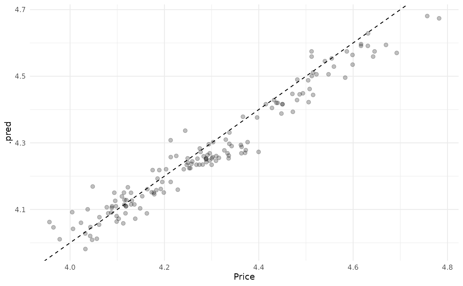
We can extract a bit of extra performance by tuning the model parameters — this is also needed if we want to stray from the default parameters when predicting ranges with the workboots package.
Tuning model parameters
Boosted tree models have a lot of available tuning parameters — given
our relatively small dataset, we’ll just focus on the mtry
and trees parameters.
# re-setup recipe with training dataset
car_rec <-
  recipe(Price ~ ., data = car_train) %>%
  step_BoxCox(Mileage) %>%
  step_dummy(all_nominal())

# setup model spec
car_spec <-
  boost_tree(
    mode = "regression",
    engine = "xgboost",
    mtry = tune(),
    trees = tune()
  )

# combine into workflow
car_wf <-
  workflow() %>%
  add_recipe(car_rec) %>%
  add_model(car_spec)

# setup cross-validation folds
set.seed(666)
car_folds <- vfold_cv(car_train)

# tune model
set.seed(555)
car_tune <-
  tune_grid(
    car_wf,
    car_folds,
    grid = 5
  )
Tuning gives us slightly better performance than the baseline model:
car_tune %>%
  show_best("rmse")
#> # A tibble: 5 × 8
#>    mtry trees .metric .estimator   mean     n std_err .config
#>   <int> <int> <chr>   <chr>       <dbl> <int>   <dbl> <chr>
#> 1     5  1545 rmse    standard   0.0446    10 0.00250 Preprocessor1_Model2
#> 2    12  1676 rmse    standard   0.0452    10 0.00241 Preprocessor1_Model4
#> 3     4   434 rmse    standard   0.0453    10 0.00247 Preprocessor1_Model1
#> 4    11   271 rmse    standard   0.0458    10 0.00241 Preprocessor1_Model3
#> 5    18  1158 rmse    standard   0.0468    10 0.00243 Preprocessor1_Model5
Now we can finalize the workflow with the best tuning parameters. With this finalized workflow, we can start predicting intervals with workboots!
car_wf_final <-
  car_wf %>%
  finalize_workflow(car_tune %>% select_best("rmse"))

car_wf_final
#> ══ Workflow ════════════════════════════════════════════════════════════════════
#> Preprocessor: Recipe
#> Model: boost_tree()
#>
#> ── Preprocessor ────────────────────────────────────────────────────────────────
#> 2 Recipe Steps
#>
#> • step_BoxCox()
#> • step_dummy()
#>
#> ── Model ───────────────────────────────────────────────────────────────────────
#> Boosted Tree Model Specification (regression)
#>
#> Main Arguments:
#>   mtry = 5
#>   trees = 1545
#>
#> Computational engine: xgboost
Predicting price ranges
To generate a prediction interval for each car’s price, we can pass
the finalized workflow to predict_boots().
library(workboots)

set.seed(444)
car_preds <-
  car_wf_final %>%
  predict_boots(
    n = 2000,
    training_data = car_train,
    new_data = car_test
  )
We can summarize the predictions with upper and lower bounds of a
prediction interval by passing car_preds to
summarise_predictions().
car_preds %>%
  summarise_predictions()
#> # A tibble: 201 × 5
#>    rowid .preds               .pred .pred_lower .pred_upper
#>    <int> <list>               <dbl>       <dbl>       <dbl>
#>  1     1 <tibble [2,000 × 2]>  4.30        4.22        4.38
#>  2     2 <tibble [2,000 × 2]>  4.48        4.41        4.55
#>  3     3 <tibble [2,000 × 2]>  4.51        4.44        4.58
#>  4     4 <tibble [2,000 × 2]>  4.44        4.37        4.51
#>  5     5 <tibble [2,000 × 2]>  4.46        4.38        4.53
#>  6     6 <tibble [2,000 × 2]>  4.50        4.41        4.57
#>  7     7 <tibble [2,000 × 2]>  4.52        4.44        4.59
#>  8     8 <tibble [2,000 × 2]>  4.52        4.45        4.59
#>  9     9 <tibble [2,000 × 2]>  4.46        4.38        4.53
#> 10    10 <tibble [2,000 × 2]>  4.46        4.38        4.53
#> # ℹ 191 more rows
How do our predictions compare against the actual values?
car_preds %>%
  summarise_predictions() %>%
  bind_cols(car_test) %>%
  ggplot(aes(x = Price,
             y = .pred,
             ymin = .pred_lower,
             ymax = .pred_upper)) +
  geom_point(size = 2,
             alpha = 0.25) +
  geom_errorbar(alpha = 0.25,
                width = 0.0125) +
  geom_abline(linetype = "dashed",
              color = "gray")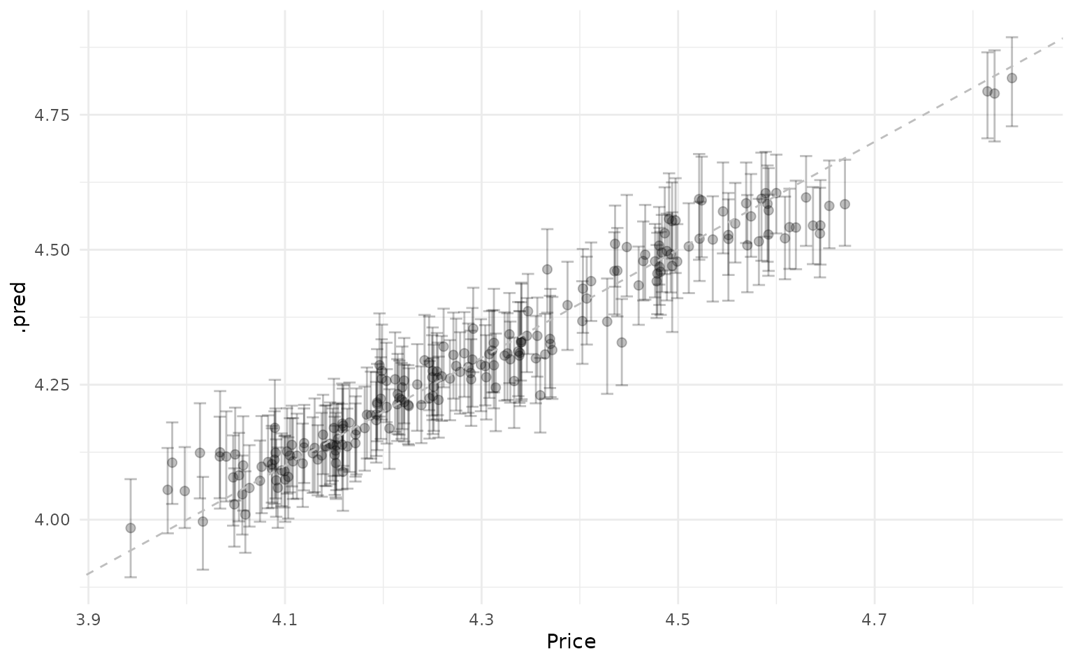
Estimating variable importance
With workboots, we can also estimate variable importance by passing
the finalized workflow to vi_boots(). This uses vip::vi()
under the hood, which doesn’t support all the model types that are
available in tidymodels — please refer to vip’s package
documentation for a full list of supported models.
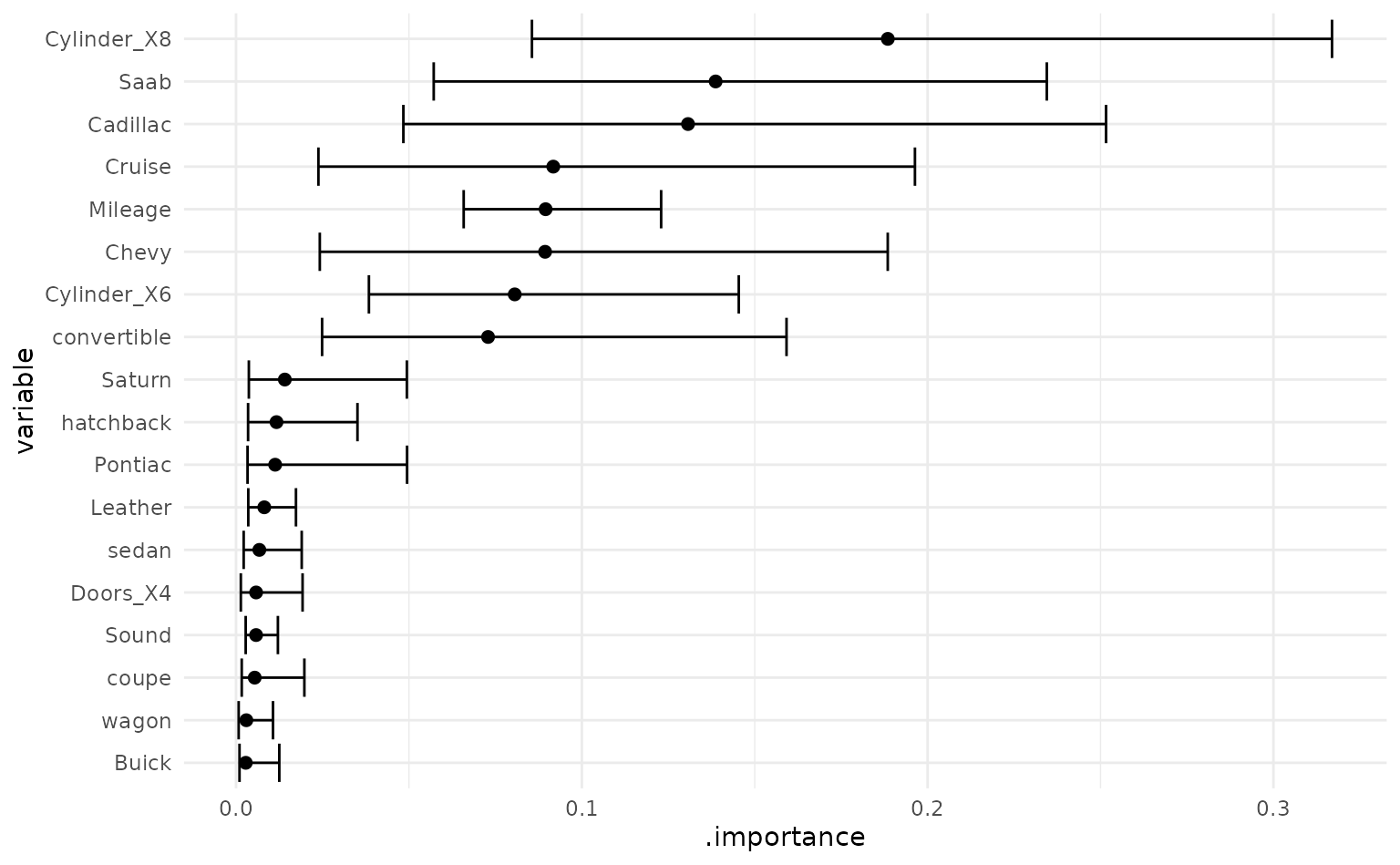
Similar to predictions, we can summarise each variable’s importance
by passing car_importance to the function
summarise_importance() and plot the results.
car_importance %>%
  summarise_importance() %>%
  mutate(variable = forcats::fct_reorder(variable, .importance)) %>%
  ggplot(aes(x = variable,
             y = .importance,
             ymin = .importance_lower,
             ymax = .importance_upper)) +
  geom_point(size = 2) +
  geom_errorbar() +
  coord_flip()