Estimating Linear Intervals

When using a linear model, we can generate prediction and confidence intervals without much effort. By way of example, we can use workboots to approximate linear model intervals. Let’s start by building a baseline model. In this example, we’ll predict a home’s sale price based on the first floor’s square footage with data from the Ames housing dataset.

library(tidymodels)

# setup our data
data("ames")
ames_mod <- ames %>% select(First_Flr_SF, Sale_Price)

# baseline plot
ames_mod %>%
  ggplot(aes(x = First_Flr_SF, y = Sale_Price)) +
  geom_point(alpha = 0.25) +
  scale_x_log10(labels = scales::comma_format()) +
  scale_y_log10(labels = scales::label_number(scale_cut = scales::cut_short_scale()))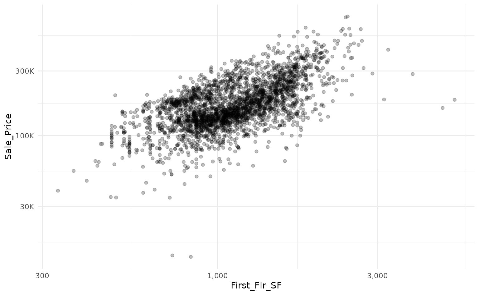

We can use a linear model to predict the log transform of Sale_Price based on the log transform of First_Flr_SFand plot our predictions against a holdout set with a prediction interval.

# log transform
ames_mod <-
  ames_mod %>%
  mutate(across(everything(), log10))

# split into train/test data
set.seed(918)
ames_split <- initial_split(ames_mod)
ames_train <- training(ames_split)
ames_test <- testing(ames_split)

# train a linear model
set.seed(314)
ames_lm <- lm(Sale_Price ~ First_Flr_SF, data = ames_train)

# predict on new data with a prediction interval
ames_lm_pred_int <-
  ames_lm %>%
  predict(ames_test, interval = "predict") %>%
  as_tibble()

ames_lm_pred_int %>%
  
  # rescale predictions to match the original dataset's scale
  bind_cols(ames_test) %>%
  mutate(across(everything(), ~10^.x)) %>%
  
  # plot!
  ggplot(aes(x = First_Flr_SF)) +
  geom_point(aes(y = Sale_Price),
             alpha = 0.25) +
  geom_line(aes(y = fit),
            size = 1) +
  geom_ribbon(aes(ymin = lwr,
                  ymax = upr),
              alpha = 0.25) +
  scale_x_log10(labels = scales::comma_format()) +
  scale_y_log10(labels = scales::label_number(scale_cut = scales::cut_short_scale()))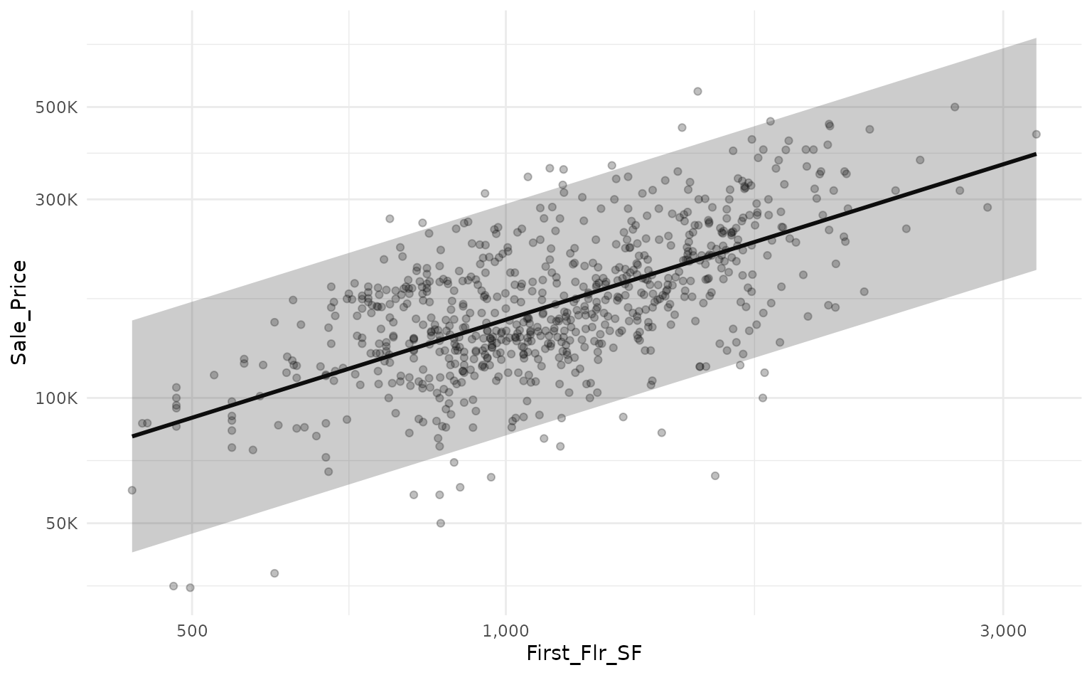

We can use workboots to approximate the linear model’s prediction interval by passing a workflow built on a linear model to predict_boots().

library(workboots)

# setup a workflow with a linear model
ames_wf <-
  workflow() %>%
  add_recipe(recipe(Sale_Price ~ First_Flr_SF, data = ames_train)) %>%
  add_model(linear_reg())

# generate bootstrap predictions on ames test
set.seed(713)
ames_boot_pred_int <- 
  ames_wf %>%
  predict_boots(
    n = 2000,
    training_data = ames_train,
    new_data = ames_test
  )

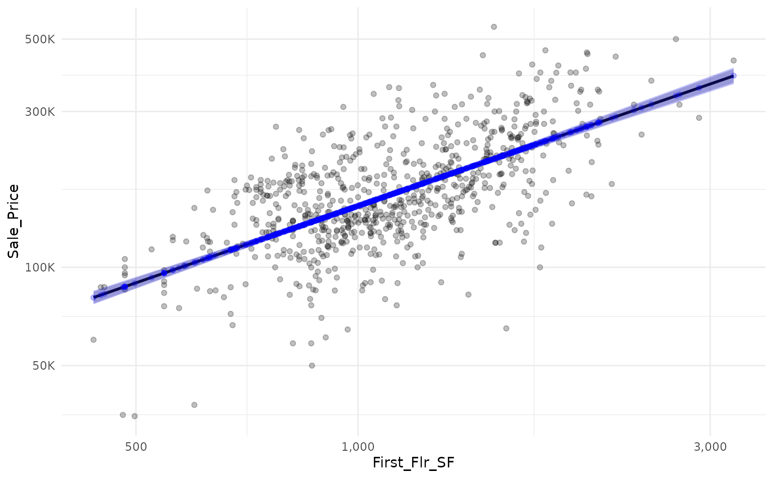
By overlaying the intervals on top of one another, we can see that the prediction interval generated by predict_boots() (in blue) is a good approximation of the theoretical interval from lm().

ames_boot_pred_int %>%
  summarise_predictions() %>%
  
  # rescale predictions to match original dataset's scale
  bind_cols(ames_lm_pred_int) %>%
  bind_cols(ames_test) %>%
  mutate(across(.pred:Sale_Price, ~10^.x)) %>%
  
  # plot!
  ggplot(aes(x = First_Flr_SF)) +
  geom_point(aes(y = Sale_Price),
             alpha = 0.25) +
  scale_x_log10(labels = scales::comma_format()) +
  scale_y_log10(labels = scales::label_number(scale_cut = scales::cut_short_scale())) +
  
  # add prediction interval created by lm()
  geom_line(aes(y = fit),
            size = 1) +
  geom_ribbon(aes(ymin = lwr,
                  ymax = upr),
              alpha = 0.25) +
  
  # add prediction interval created by workboots
  geom_point(aes(y = .pred),
             color = "blue",
             alpha = 0.25) +
  geom_errorbar(aes(ymin = .pred_lower,
                    ymax = .pred_upper),
                color = "blue",
                alpha = 0.25,
                width = 0.0125)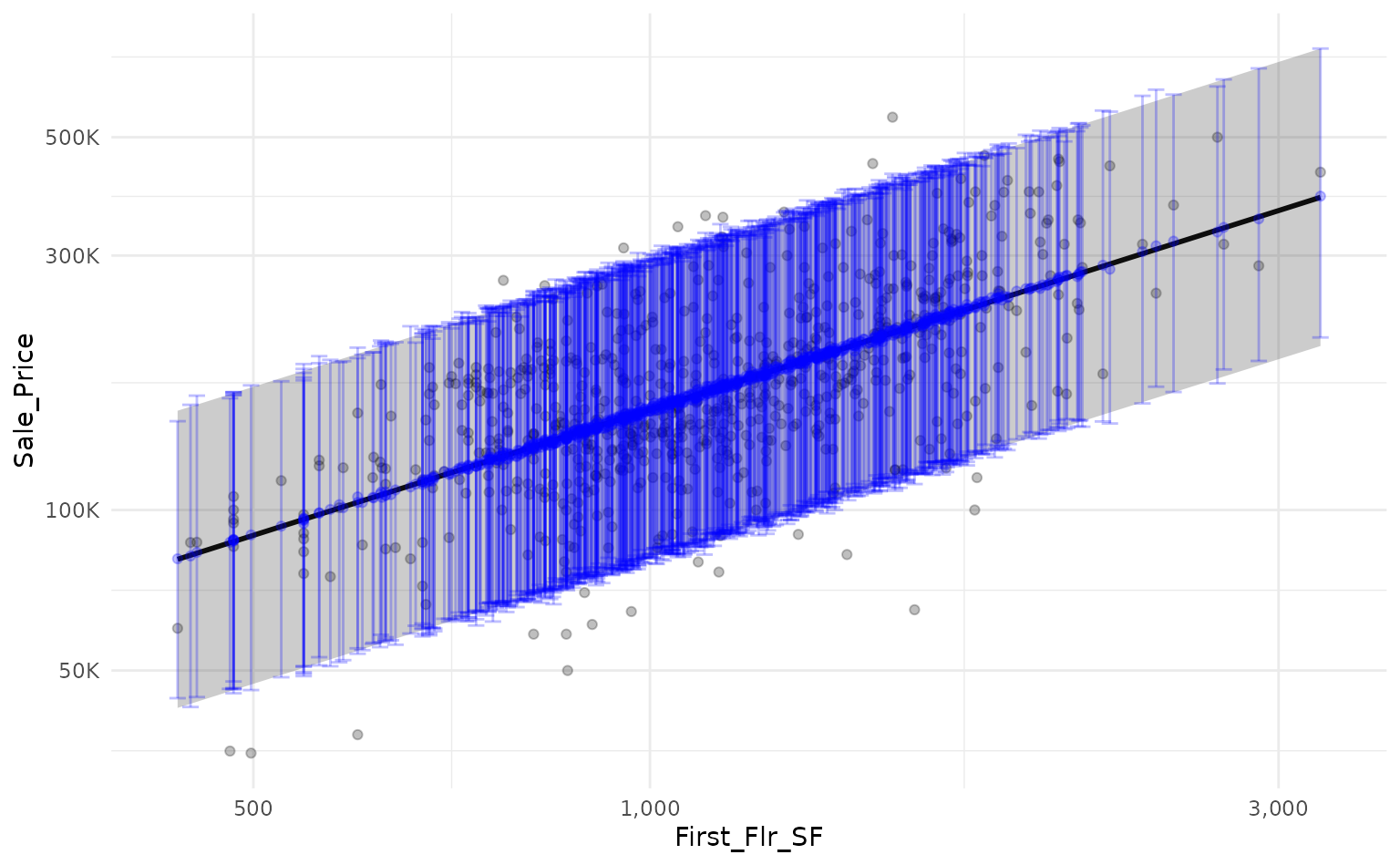

Both lm() and summarise_predictions() use a 95% prediction interval by default but we can generate other intervals by passing different values to the parameter interval_width:

ames_boot_pred_int %>%
  
  # generate a 95% prediction interval
  summarise_predictions(interval_width = 0.95) %>%
  rename(.pred_lower_95 = .pred_lower,
         .pred_upper_95 = .pred_upper) %>%
  select(-.pred) %>%
  
  # generate 80% prediction interval
  summarise_predictions(interval_width = 0.80) %>%
  rename(.pred_lower_80 = .pred_lower,
         .pred_upper_80 = .pred_upper) %>%
  
  # rescale predictions to match original dataset's scale
  bind_cols(ames_test) %>%
  mutate(across(.pred_lower_95:Sale_Price, ~10^.x)) %>%
  
  # plot!
  ggplot(aes(x = First_Flr_SF)) +
  geom_point(aes(y = Sale_Price),
             alpha = 0.25) +
  geom_line(aes(y = .pred),
            size = 1,
            color = "blue") +
  geom_ribbon(aes(ymin = .pred_lower_95,
                  ymax = .pred_upper_95),
              alpha = 0.25,
              fill = "blue") +
  geom_ribbon(aes(ymin = .pred_lower_80,
                  ymax = .pred_upper_80),
              alpha = 0.25,
              fill = "blue") +
  scale_x_log10(labels = scales::comma_format()) +
  scale_y_log10(labels = scales::label_number(scale_cut = scales::cut_short_scale()))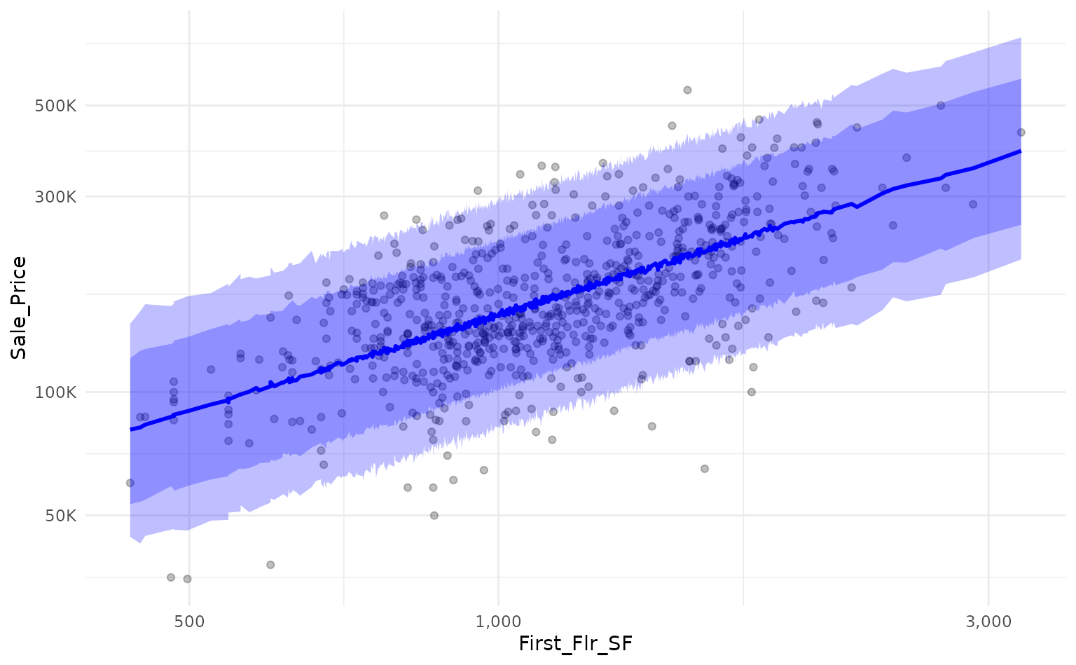

Alternatively, we can estimate the confidence interval around each prediction by passing the argument "confidence" to the interval parameter of predict_boots().

# generate linear model confidence interval for reference
ames_lm_conf_int <-
  ames_lm %>%
  predict(ames_test, interval = "confidence") %>%
  as_tibble()

# generate bootstrap predictions on test set
set.seed(867)
ames_boot_conf_int <-
  ames_wf %>%
  predict_boots(
    n = 2000,
    training_data = ames_train,
    new_data = ames_test,
    interval = "confidence"
  )

Again, by overlaying the intervals on the same plot, we can see that the confidence interval generated by predict_boots() is a good approximation of the theoretical interval.

ames_boot_conf_int %>%
  summarise_predictions() %>%
  
  # rescale predictions to match original dataset's scale
  bind_cols(ames_lm_conf_int) %>%
  bind_cols(ames_test) %>%
  mutate(across(.pred:Sale_Price, ~10^.x)) %>%

  # plot!
  ggplot(aes(x = First_Flr_SF)) +
  geom_point(aes(y = Sale_Price),
             alpha = 0.25) +
  scale_x_log10(labels = scales::comma_format()) +
  scale_y_log10(labels = scales::label_number(scale_cut = scales::cut_short_scale())) +
  
  # add prediction interval created by lm()
  geom_line(aes(y = fit),
            size = 1) +
  geom_ribbon(aes(ymin = lwr,
                  ymax = upr),
              alpha = 0.25) +
  
  # add prediction interval created by workboots
  geom_point(aes(y = .pred),
             color = "blue",
             alpha = 0.25) +
  geom_ribbon(aes(ymin = .pred_lower,
                  ymax = .pred_upper),
              fill = "blue",
              alpha = 0.25)